12. Optimal Taxation in an LQ Economy#

12.1.1. Model Features#

• Linear quadratic (LQ) model

• Representative household

• Stochastic dynamic programming over an infinite horizon

• Distortionary taxation

12.2.1. Technology#

Labor can be converted one-for-one into a single, non-storable consumption good.

In the usual spirit of the LQ model, the amount of labor supplied in each period is unrestricted.

This is unrealistic, but helpful when it comes to solving the model.

Realistic labor supply can be induced by suitable parameter values.

12.2.2. Households#

Consider a representative household who chooses a path $\{{\ell }_t,c_t\}$ for labor and consumption to maximize

subject to the budget constraint

Here

• $\beta$ is a discount factor in $(0,1)$.

• $p_t^0$ is a scaled Arrow-Debreu price at time $0$ of history contingent goods at time $t+j$.

• $b_t$ is a stochastic preference parameter.

• $d_t$ is an endowment process.

• ${\tau }_t$ is a flat tax rate on labor income.

• $s_t$ is a promised time-$t$ coupon payment on debt issued by the government.

The scaled Arrow-Debreu price $p_t^0$ is related to the unscaled Arrow-Debreu price as follows.

If we let ${\pi }_t^0(x^t)$ denote the probability (density) of a history $x^t=[x_t,x_{t-1},\dots ,x_0]$ of the state $x^t$, then the Arrow-Debreu time $0$ price of a claim on one unit of consumption at date $t$, history $x^t$ would be

Thus, our scaled Arrow-Debreu price is the ordinary Arrow-Debreu price multiplied by the discount factor ${\beta }^t$ and divided by an appropriate probability.

The budget constraint (12.2) requires that the present value of consumption be restricted to equal the present value of endowments, labor income and coupon payments on bond holdings.

12.2.3. Government#

The government imposes a linear tax on labor income, fully committing to a stochastic path of tax rates at time zero.

The government also issues state-contingent debt.

Given government tax and borrowing plans, we can construct a competitive equilibrium with distorting government taxes.

Among all such competitive equilibria, the Ramsey plan is the one that maximizes the welfare of the representative consumer.

12.2.4. Exogenous Variables#

Endowments, government expenditure, the preference shock process $b_t$, and promised coupon payments on initial government debt $s_t$ are all exogenous, and given by

• $d_t=S_d{x}_t$

• $g_t=S_g{x}_t$

• $b_t=S_b{x}_t$

• $s_t=S_s{x}_t$

The matrices $S_d,S_g,S_b,S_s$ are primitives and $\{x_t\}$ is an exogenous stochastic process taking values in ${\mathbb{R}}^k$.

We consider two specifications for $\{x_t\}$.

1. Discrete case: $\{x_t\}$ is a discrete state Markov chain with transition matrix $P$.

2. VAR case: $\{x_t\}$ obeys $x_{t+1}=A{x}_t+C{w}_{t+1}$ where $\{w_t\}$ is independent zero-mean Gaussian with identify covariance matrix.

12.2.5. Feasibility#

The period-by-period feasibility restriction for this economy is

A labor-consumption process $\{{\ell }_t,c_t\}$ is called feasible if (12.3) holds for all $t$.

12.2.6. Government Budget Constraint#

Where $p_t^0$ is again a scaled Arrow-Debreu price, the time zero government budget constraint is

12.2.7. Equilibrium#

An equilibrium is a feasible allocation $\{{\ell }_t,c_t\}$, a sequence of prices $\{p_t^0\}$, and a tax system $\{{\tau }_t\}$ such that

1. The allocation $\{{\ell }_t,c_t\}$ is optimal for the household given $\{p_t^0\}$ and $\{{\tau }_t\}$.

2. The government’s budget constraint (12.4) is satisfied.

The Ramsey problem is to choose the equilibrium $\{{\ell }_t,c_t,{\tau }_t,p_t^0\}$ that maximizes the household’s welfare.

If $\{{\ell }_t,c_t,{\tau }_t,p_t^0\}$ solves the Ramsey problem, then $\{{\tau }_t\}$ is called the Ramsey plan.

The solution procedure we adopt is

1. Use the first-order conditions from the household problem to pin down prices and allocations given $\{{\tau }_t\}$.

2. Use these expressions to rewrite the government budget constraint (12.4) in terms of exogenous variables and allocations.

3. Maximize the household’s objective function (12.1) subject to the constraint constructed in step 2 and the feasibility constraint (12.3).

The solution to this maximization problem pins down all quantities of interest.

12.2.8. Solution#

Step one is to obtain the first-conditions for the household’s problem, taking taxes and prices as given.

Letting $\mu$ be the Lagrange multiplier on (12.2), the first-order conditions are $p_t^0=(c_t-b_t)/\mu$ and ${\ell }_t=(c_t-b_t)(1-{\tau }_t)$.

Rearranging and normalizing at $\mu =b_0-c_0$, we can write these conditions as

Substituting (12.5) into the government’s budget constraint (12.4) yields

The Ramsey problem now amounts to maximizing (12.1) subject to (12.6) and (12.3).

The associated Lagrangian is

The first-order conditions associated with $c_t$ and ${\ell }_t$ are

and

Combining these last two equalities with (12.3) and working through the algebra, one can show that

where

• $\nu :=\lambda /(1+2\lambda )$

• ${\overline{\ell }}_t:=(b_t-d_t+g_t)/2$

• ${\overline{c}}_t:=(b_t+d_t-g_t)/2$

• $m_t:=(b_t-d_t-s_t)/2$

Apart from $\nu$, all of these quantities are expressed in terms of exogenous variables.

To solve for $\nu$, we can use the government’s budget constraint again.

The term inside the brackets in (12.6) is $(b_t-c_t)(s_t+g_t)-(b_t-c_t){\ell }_t+{\ell }_t^2$.

Using (12.8), the definitions above and the fact that $\overline{\ell }=b-\overline{c}$, this term can be rewritten as

Reinserting into (12.6), we get

Although it might not be clear yet, we are nearly there because:

• The two expectations terms in (12.9) can be solved for in terms of model primitives.

• This in turn allows us to solve for the Lagrange multiplier $\nu$.

• With $\nu$ in hand, we can go back and solve for the allocations via (12.8).

• Once we have the allocations, prices and the tax system can be derived from (12.5).

12.2.9. Computing the Quadratic Term#

Let’s consider how to obtain the term $\nu$ in (12.9).

If we can compute the two expected geometric sums

then the problem reduces to solving

for $\nu$.

Provided that $4b_0<a_0$, there is a unique solution $\nu \in (0,1/2)$, and a unique corresponding $\lambda >0$.

Let’s work out how to compute mathematical expectations in (12.10).

For the first one, the random variable $(b_t-{\overline{c}}_t)(g_t+s_t)$ inside the summation can be expressed as

For the second expectation in (12.10), the random variable $2m_t^2$ can be written as

It follows that both objects of interest are special cases of the expression

where $H$ is a matrix conformable to $x_t$ and $x_t^{\prime }$ is the transpose of column vector $x_t$.

Suppose first that $\{x_t\}$ is the Gaussian VAR described above.

In this case, the formula for computing $q(x_0)$ is known to be $q(x_0)=x_0^{\prime }Q{x}_0+v$, where

• $Q$ is the solution to $Q=H+\beta A^{\prime }QA$, and

• $v=\text{trace}(C^{\prime }QC)\beta /(1-\beta )$

The first equation is known as a discrete Lyapunov equation and can be solved using this function.

12.2.10. Finite State Markov Case#

Next, suppose that $\{x_t\}$ is the discrete Markov process described above.

Suppose further that each $x_t$ takes values in the state space $\{x^1,\dots ,x^N\}\subset {\mathbb{R}}^k$.

Let $h:{\mathbb{R}}^k\to \mathbb{R}$ be a given function, and suppose that we wish to evaluate

For example, in the discussion above, $h(x_t)=x_t^{\prime }H{x}_t$.

It is legitimate to pass the expectation through the sum, leading to

Here

• $P^t$ is the $t$-th power of the transition matrix $P$.

• $h$ is, with some abuse of notation, the vector $(h(x^1),\dots ,h(x^N))$.

• $(P^{t}h)[j]$ indicates the $j$-th element of $P^{t}h$.

It can be shown that (12.12) is in fact equal to the $j$-th element of the vector $(I-\beta P{)}^{-1}h$.

This last fact is applied in the calculations below.

12.2.11. Other Variables#

We are interested in tracking several other variables besides the ones described above.

To prepare the way for this, we define

as the scaled Arrow-Debreu time $t$ price of a history contingent claim on one unit of consumption at time $t+j$.

These are prices that would prevail at time $t$ if markets were reopened at time $t$.

These prices are constituents of the present value of government obligations outstanding at time $t$, which can be expressed as

Using our expression for prices and the Ramsey plan, we can also write $B_t$ as

This version is more convenient for computation.

Using the equation

it is possible to verify that (12.13) implies that

and

Define

$R_t$ is the gross $1$-period risk-free rate for loans between $t$ and $t+1$.

12.2.12. A Martingale#

We now want to study the following two objects, namely,

and the cumulation of ${\pi }_t$

The term ${\pi }_{t+1}$ is the difference between two quantities:

• $B_{t+1}$, the value of government debt at the start of period $t+1$.

• $R_t[B_t+g_t-{\tau }_t]$, which is what the government would have owed at the beginning of period $t+1$ if it had simply borrowed at the one-period risk-free rate rather than selling state-contingent securities.

Thus, ${\pi }_{t+1}$ is the excess payout on the actual portfolio of state-contingent government debt relative to an alternative portfolio sufficient to finance $B_t+g_t-{\tau }_t{\ell }_t$ and consisting entirely of risk-free one-period bonds.

Use expressions (12.14) and (12.15) to obtain

or

where ${\tilde{E}}_t$ is the conditional mathematical expectation taken with respect to a one-step transition density that has been formed by multiplying the original transition density with the likelihood ratio

It follows from equation (12.16) that

which asserts that $\{{\pi }_{t+1}\}$ is a martingale difference sequence under the distorted probability measure, and that $\{{\mathrm{\Pi }}_t\}$ is a martingale under the distorted probability measure.

In the tax-smoothing model of Robert Barro [Barro, 1979], government debt is a random walk.

In the current model, government debt $\{B_t\}$ is not a random walk, but the excess payoff $\{{\mathrm{\Pi }}_t\}$ on it is.

12.3.1. Comments on the Code#

The function var_quadratic_sum imported from quadsums is for computing the value of (12.11) when the exogenous process $\{x_t\}$ is of the VAR type described above.

Below the definition of the function, you will see definitions of two namedtuple objects, Economy and Path.

The first is used to collect all the parameters and primitives of a given LQ economy, while the second collects output of the computations.

In Python, a namedtuple is a popular data type from the collections module of the standard library that replicates the functionality of a tuple, but also allows you to assign a name to each tuple element.

These elements can then be references via dotted attribute notation — see for example the use of path in the functions gen_fig_1() and gen_fig_2().

The benefits of using namedtuples:

• Keeps content organized by meaning.

• Helps reduce the number of global variables.

Other than that, our code is long but relatively straightforward.

12.4.1. The Continuous Case#

Our first example adopts the VAR specification described above.

Regarding the primitives, we set

• $\beta =1/1.05$

• $b_t=2.135$ and $s_t=d_t=0$ for all $t$

Government spending evolves according to

with $\rho =0.7$, ${\mu }_g=0.35$ and $C_g={\mu }_g\sqrt{1-{\rho }^2}/10$.

Here’s the code

# == Parameters == #
β = 1 / 1.05
ρ, mg = .7, .35
A = eye(2)
A[0, :] = ρ, mg * (1-ρ)
C = np.zeros((2, 1))
C[0, 0] = np.sqrt(1 - ρ**2) * mg / 10
Sg = np.array((1, 0)).reshape(1, 2)
Sd = np.array((0, 0)).reshape(1, 2)
Sb = np.array((0, 2.135)).reshape(1, 2)
Ss = np.array((0, 0)).reshape(1, 2)

economy = Economy(β=β, Sg=Sg, Sd=Sd, Sb=Sb, Ss=Ss,
                discrete=False, proc=(A, C))

T = 50
path = compute_paths(T, economy)
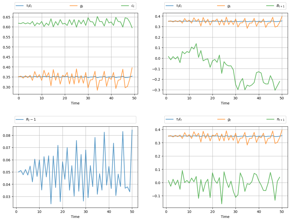
gen_fig_1(path)

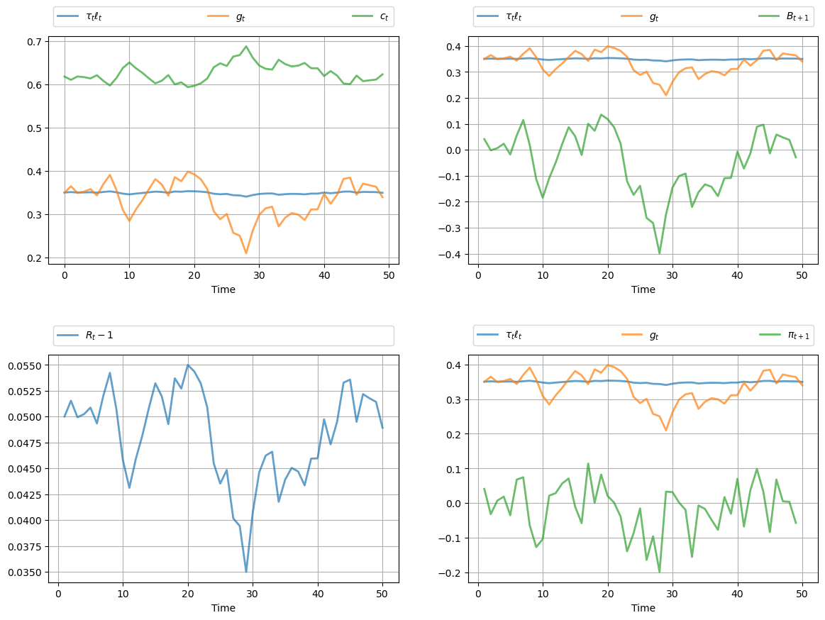
The legends on the figures indicate the variables being tracked.

Most obvious from the figure is tax smoothing in the sense that tax revenue is much less variable than government expenditure.

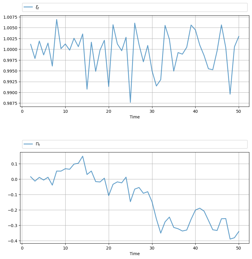
gen_fig_2(path)

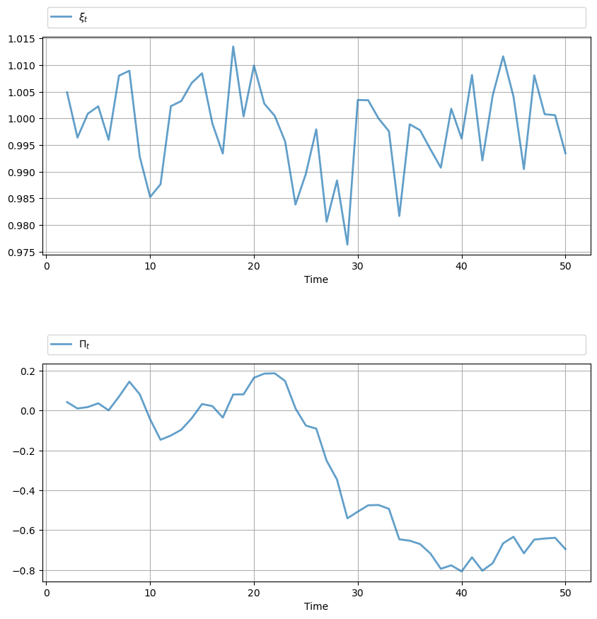
See the original manuscript for comments and interpretation.

12.4.2. The Discrete Case#

Our second example adopts a discrete Markov specification for the exogenous process

# == Parameters == #
β = 1 / 1.05
P = np.array([[0.8, 0.2, 0.0],
            [0.0, 0.5, 0.5],
            [0.0, 0.0, 1.0]])

# Possible states of the world
# Each column is a state of the world. The rows are [g d b s 1]
x_vals = np.array([[0.5, 0.5, 0.25],
                [0.0, 0.0,  0.0],
                [2.2, 2.2,  2.2],
                [0.0, 0.0,  0.0],
                [1.0, 1.0,  1.0]])

Sg = np.array((1, 0, 0, 0, 0)).reshape(1, 5)
Sd = np.array((0, 1, 0, 0, 0)).reshape(1, 5)
Sb = np.array((0, 0, 1, 0, 0)).reshape(1, 5)
Ss = np.array((0, 0, 0, 1, 0)).reshape(1, 5)

economy = Economy(β=β, Sg=Sg, Sd=Sd, Sb=Sb, Ss=Ss,
                discrete=True, proc=(P, x_vals))

T = 15
path = compute_paths(T, economy)
gen_fig_1(path)

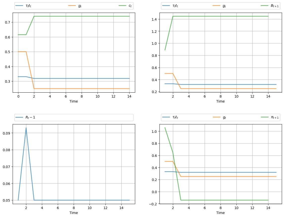
The call gen_fig_2(path) generates

gen_fig_2(path)

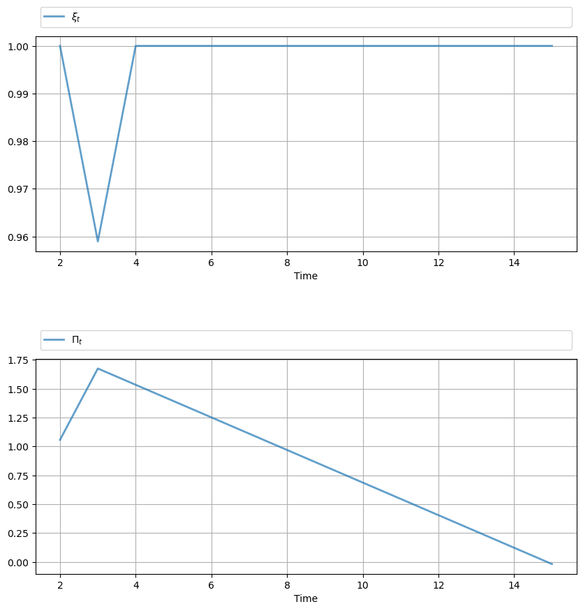
See the original manuscript for comments and interpretation.