40. Optimal Unemployment Insurance#

40.1. Overview#

This lecture describes a model of optimal unemployment insurance created by Shavell and Weiss (1979) [Shavell and Weiss, 1979].

We use recursive techniques of Hopenhayn and Nicolini (1997) [Hopenhayn and Nicolini, 1997] to compute optimal insurance plans for Shavell and Weiss’s model.

Hopenhayn and Nicolini’s model is a generalization of Shavell and Weiss’s along dimensions that we’ll soon describe.

40.2. Shavell and Weiss’s Model#

An unemployed worker orders stochastic processes of consumption and search effort ${c_{t}, a_{t}}_{t = 0}^{\infty}$ according to

(40.1)#

E \sum_{t = 0}^{\infty} β^{t} [u (c_{t}) - a_{t}]

where $β \in (0, 1)$ and $u (c)$ is strictly increasing, twice differentiable, and strictly concave.

We assume that $u (0)$ is well defined.

We require that $c_{t} \geq 0$ and $a_{t} \geq 0$ .

All jobs are alike and pay wage $w > 0$ units of the consumption good each period forever.

An unemployed worker searches with effort $a$ and with probability $p (a)$ receives a permanent job at the beginning of the next period.

Furthermore, $a = 0$ when the worker is employed.

The probability of finding a job is $p (a)$ .

$p$ is an increasing, strictly concave, and twice differentiable function of $a$ that satisfies $p (a) \in [0, 1]$ for $a \geq 0$ , $p (0) = 0$ .

Note

When we compute examples below, we’ll use assume the same $p (a)$ function as [Hopenhayn and Nicolini, 1997], namely, $p (a) = 1 - \exp (- r a)$ , where $r$ is a parameter that we’ll calibrate to hit the same target that [Hopenhayn and Nicolini, 1997] did, namely, an empirical hazard rate of leaving unemployment.

The consumption good is nonstorable.

An unemployed worker has no savings and cannot borrow or lend.

The unemployed worker’s only source of consumption smoothing over time and across states is an insurance agency or planner.

Once a worker has found a job, he is beyond the planner’s grasp.

This is Shavell and Weiss’s assumption, but not Hopenhayn and Nicolini’s.
Hopenhayn and Nicolini allow the unemployment insurance agency to impose history-dependent taxes on previously unemployed workers.
Since there is no incentive problem after the worker has found a job, it is optimal for the agency to provide an employed worker with a constant level of consumption.
Hence, Hopenhayn and Nicolini’s insurance agency imposes a permanent per-period history-dependent tax on a previously unemployed but presently employed worker.

40.2.1. Autarky#

As a benchmark, we first study the fate of an unemployed worker who has no access to unemployment insurance.

Because employment is an absorbing state for the worker, we work backward from that state.

Let $V^{e}$ be the expected sum of discounted one-period utilities of an employed worker.

Once the worker is employed, $a = 0$ , making his period utility be $u (c) - a = u (w)$ forever.

Therefore,

(40.2)#

V^{e} = \frac{u (w)}{(1 - β)} .

Now let $V^{u}$ be the expected discounted present value of utility for an unemployed worker who chooses consumption, effort pair $(c, a)$ optimally.

Value $V^{u}$ satisfies the Bellman equation

(40.3)#

V^{u} = max_{a \geq 0} {u (0) - a + β [p (a) V^{e} + (1 - p (a)) V^{u}]} .

The first-order condition for a maximum is

(40.4)#

β p^{'} (a) [V^{e} - V^{u}] \leq 1,

with equality if $a > 0$ .

Since there is no state variable in this infinite horizon problem, there is a time-invariant optimal search intensity $a$ and an associated value of being unemployed $V^{u}$ .

Let $V_{a u t} = V^{u}$ solve Bellman equation (40.3).

Equations (40.3) and (40.4) form the basis for an iterative algorithm for computing $V^{u} = V_{a u t}$ .

Let $V_{j}^{u}$ be the estimate of $V_{a u t}$ at the $j$ th iteration.
Use this value in equation (40.4) and solve for an estimate of effort $a_{j}$ .
Use this value in a version of equation (40.3) with $V_{j}^{u}$ on the right side to compute $V_{j + 1}^{u}$ .
Iterate to convergence.

40.2.2. Full Information#

Another benchmark model helps set the stage for the model with private information that we ultimately want to study.

We temporarily assume that an unemployment insurance agency has full information about the unemployed worker.

We assume that the insurance agency can control both the consumption and the search effort of an unemployed worker.

The agency wants to design an unemployment insurance contract to give the unemployed worker expected discounted utility $V > V_{a u t}$ .

The agency, i.e., the planner, wants to deliver value $V$ efficiently, meaning in a way that minimizes an expected present value discounted costs, using $β$ as the discount factor.

We formulate the optimal insurance problem recursively.

Let $C (V)$ be the expected discounted cost of giving the worker expected discounted utility $V$ .

The cost function is strictly convex because a higher $V$ implies a lower marginal utility of the worker; that is, additional expected utils can be awarded to the worker only at an increasing marginal cost in terms of the consumption good.

Given $V$ , the planner assigns first-period pair $(c, a)$ and promised continuation value $V^{u}$ next period if the worker is unlucky and does not find a job this period.

The planner sets $(c, a, V^{u})$ as functions of $V$ and to satisfy the following Bellman equation for associated cost function $C (V)$ :

(40.5)#

C (V) = min_{c, a, V^{u}} {c + β [1 - p (a)] C (V^{u})},

where minimization is subject to the promise-keeping constraint

(40.6)#

V \leq u (c) - a + β {p (a) V^{e} + [1 - p (a)] V^{u}} .

Here $V^{e}$ is given by equation (40.2), which reflects the assumption that once the worker is employed, he is beyond the reach of the unemployment insurance agency.

The right side of Bellman equation (40.5) is attained by policy functions $c = c (V), a = a (V)$ , and $V^{u} = V^{u} (V)$ .

The promise-keeping constraint, equation (40.6), asserts that the 3-tuple $(c, a, V^{u})$ attains at least $V$ .

Let $θ$ be a Lagrange multiplier on constraint (40.6).

At an interior solution, first-order conditions with respect to $c, a$ , and $V^{u}$ , respectively, are

(40.7)#

\begin{aligned} θ & = \frac{1}{u^{'} (c)}, \\ C (V^{u}) & = θ [\frac{1}{β p^{'} (a)} - (V^{e} - V^{u})], \\ C^{'} (V^{u}) & = θ . \end{aligned}

The envelope condition $C^{'} (V) = θ$ and the third equation of (40.7) imply that $C^{'} (V^{u}) = C^{'} (V)$ .

Strict convexity of $C$ then implies that $V^{u} = V$ .

Applied repeatedly over time, $V^{u} = V$ makes the continuation value remain constant during the entire spell of unemployment.

The first equation of (40.7) determines $c$ , and the second equation of (40.7) determines $a$ , both as functions of promised value $V$ .

That $V^{u} = V$ then implies that $c$ and $a$ are held constant during the unemployment spell.

Thus, the unemployed worker’s consumption $c$ and search effort $a$ are both fully smoothed during the unemployment spell.

But the worker’s consumption is not smoothed across states of employment and unemployment unless $V = V^{e}$ .

40.2.3. Incentive Problem#

The preceding efficient insurance scheme assumes that the insurance agency controls both $c$ and $a$ .

The insurance agency cannot simply provide $c$ and then allow the worker to choose $a$ .

Here is why.

The agency delivers a value $V^{u}$ higher than the autarky value $V_{a u t}$ by doing two things.

It increases the unemployed worker’s consumption $c$ and decreases his search effort $a$ .

The prescribed search effort is higher than what the worker would choose if he were to be guaranteed consumption level $c$ while he remains unemployed.

This follows from the first two equations of (40.7) and the fact that the insurance scheme is costly, $C (V^{u}) > 0$ , which imply $[β p^{'} (a)]^{- 1} > (V^{e} - V^{u})$ .

Now look at the worker’s first-order condition (40.4) under autarky.

It implies that if search effort $a > 0$ , then $[β p^{'} (a)]^{- 1} = [V^{e} - V^{u}]$ , which is inconsistent with the inequality $[β p^{'} (a)]^{- 1} > (V^{e} - V^{u})$ that prevails when $a > 0$ when the agency controls both $a$ and $c$ .

If he were free to choose $a$ , the worker would therefore want to fulfill (40.4), either at equality so long as $a > 0$ , or by setting $a = 0$ otherwise.

Starting from the $a$ associated with the full-information social insurance scheme in which the agency controls both $c$ and $a$ , the worker would establish the desired equality in (40.4) by lowering $a$ , thereby decreasing the term $[β p^{'} (a)]^{- 1}$ (which also lowers $(V^{e} - V^{u})$ when the value of being unemployed $V^{u}$ increases).

If an equality can be established before $a$ reaches zero, this would be the worker’s preferred search effort; otherwise the worker would find it optimal to accept the insurance payment, set $a = 0$ , and never work again.

Thus, since the worker does not take the cost of the insurance scheme into account, he would choose a search effort below the socially optimal, full-information level.

The full-information contract thus relies on the agency’s ability to control both the unemployed worker’s consumption and his search effort.

40.3. Private Information#

Following [Shavell and Weiss, 1979] and [Hopenhayn and Nicolini, 1997], now assume that the unemployment insurance agency cannot observe or control $a$ , though it can observe and control $c$ .

The worker is free to choose $a$ , which puts expression (40.4), the worker’s first-order condition under autarky, back in the picture.

We are assuming that the worker’s best response to the unemployment insurance arrangement is completely characterized by the first-order condition (40.4), an instance of the so-called first-order approach to incentive problems.

Given a contract, the individual will choose search effort according to first-order condition (40.4).

This fact motivates the insurance agency to design an unemployment insurance contract that respects this restriction.

Thus, the contract design problem is now to minimize the right side of equation (40.5) subject to expression (40.6) and the incentive constraint (40.4).

Since the restrictions (40.4) and (40.6) are not linear and generally do not define a convex set, it becomes challenging to provide conditions under which the solution to the dynamic programming problem results in a convex function $C (V)$ .

Sometimes this complication can be handled by convexifying the constraint set by introducing lotteries.
A common finding is that optimal plans do not involve lotteries, because convexity of the constraint set is a sufficient but not necessary condition for convexity of the cost function.
In order to characterize the optimal solution, we follow Hopenhayn and Nicolini (1997) [Hopenhayn and Nicolini, 1997] by hopefully proceeding under the assumption that $C (V)$ is strictly convex.

Let $η$ be the multiplier on constraint (40.4), while $θ$ continues to denote the multiplier on constraint (40.6).

But now we replace the weak inequality in (40.6) by an equality.

We do this because the unemployment insurance agency cannot award a higher utility than $V$ because that might violate an incentive-compatibility constraint for exerting the proper search effort in earlier periods.

At an interior solution, first-order conditions with respect to $c, a$ , and $V^{u}$ , respectively, are

(40.8)#

\begin{aligned} θ & = \frac{1}{u^{'} (c)}, \\ C (V^{u}) & = θ [\frac{1}{β p^{'} (a)} - (V^{e} - V^{u})] - η \frac{p^{″} (a)}{p^{'} (a)} (V^{e} - V^{u}) \\ = - η \frac{p^{″} (a)}{p^{'} (a)} (V^{e} - V^{u}), \\ C^{'} (V^{u}) & = θ - η \frac{p^{'} (a)}{1 - p (a)}, \end{aligned}

where the second equality in the second equation in (40.8) follows from strict equality of the incentive constraint (40.4) when $a > 0$ .

As long as the insurance scheme is associated with costs, so that $C (V^{u}) > 0$ , the first-order condition in the second equation of (40.8) implies that the multiplier $η$ is strictly positive.

The first-order condition in the second equation of the third equality in (40.8) and the envelope condition $C^{'} (V) = θ$ together allow us to conclude that $C^{'} (V^{u}) < C^{'} (V)$ .

Convexity of $C$ then implies that $V^{u} < V$ .

After we have also used the first equation of (40.8), it follows that in order to provide the proper incentives, the consumption of the unemployed worker must decrease as the duration of the unemployment spell lengthens.

It also follows from (40.4) at equality that search effort $a$ rises as $V^{u}$ falls, i.e., it rises with the duration of unemployment.

The of benefits on the duration of unemployment is designed to provide the worker an incentive to search.

To understand this, from the third equation of (40.8), notice how the conclusion that consumption falls with the duration of unemployment depends on the assumption that more search effort raises the prospect of finding a job, i.e., that $p^{'} (a) > 0$ .

If $p^{'} (a) = 0$ , then the third equation of (40.8) and the strict convexity of $C$ imply that $V^{u} = V$ .

Thus, when $p^{'} (a) = 0$ , there is no reason for the planner to make consumption fall with the duration of unemployment.

40.3.1. Computational Details#

It is useful to note that there are natural lower and upper bounds to the set of continuation values $V^{u}$ .

The lower bound is the expected lifetime utility in autarky, $V_{a u t}$ .

To compute an upper bound, represent condition (40.4) as

V^{u} \geq V^{e} - [β p^{'} (a)]^{- 1},

with equality if $a > 0$ .

If there is zero search effort, then $V^{u} \geq V^{e} - [β p^{'} (0)]^{- 1}$ .

Therefore, to rule out zero search effort we require

V^{u} < V^{e} - [β p^{'} (0)]^{- 1} .

(Remember that $p^{″} (a) < 0$ .)

This step gives our upper bound for $V^{u}$ .

To formulate the Bellman equation numerically, we suggest using the constraints to eliminate $c$ and $a$ as choice variables, thereby reducing the Bellman equation to a minimization over the one choice variable $V^{u}$ .

First express the promise-keeping constraint (40.6) at equality as

u (c) = V + a - β {p (a) V^{e} + [1 - p (a)] V^{u}}

so that consumption is

(40.9)#

c = u^{- 1} (V + a - β [p (a) V^{e} + (1 - p (a)) V^{u}]) .

Similarly, solving the inequality (40.4) for $a$ leads to

(40.10)#

a = max {0, p^{' - 1} (\frac{1}{β (V^{e} - V^{u})})} .

When we specialize (40.10) to the functional form for $p (a)$ used by Hopenhayn and Nicolini, we obtain

(40.11)#

a = max {0, \frac{\log [r β (V^{e} - V^{u})]}{r}} .

Formulas (40.9) and (40.11) express $(c, a)$ as functions of $V$ and the continuation value $V^{u}$ .

Using these functions allows us to write the Bellman equation in $C (V)$ as

(40.12)#

C (V) = min_{V^{u}} {c + β [1 - p (a)] C (V^{u})}

where $c$ and $a$ are given by equations (40.9) and (40.11).

40.3.2. Python Computations#

We’ll approximate the planner’s optimal cost function with cubic splines.

To do this, we’ll load some useful modules

import numpy as np
import scipy as sp
import matplotlib.pyplot as plt

We first create a class to set up a particular parametrization.

class params_instance:

    def __init__(self,
                r,
                β = 0.999,
                σ = 0.500,
                w = 100,
                n_grid = 50):

        self.β,self.σ,self.w,self.r = β,σ,w,r
        self.n_grid = n_grid
        uw = self.w**(1-self.σ)/(1-self.σ)  #Utility from consuming all wage
        self.Ve = uw/(1-β)

40.3.3. Parameter Values#

For the other parameters appearing in the above Python code, we’ll calibrate parameter $r$ that pins down the function $p (a) = 1 - \exp (- r a)$ to match an observerd hazard rate – the probability that an unemployed worker finds a job each – in US data.

In particular, we seek an $r$ so that in autarky p(a(r)) = 0.1, where a is the optimal search effort.

First, we create some helper functions.

# The probability of finding a job given search effort, a and parameter r.
def p(a,r):
    return 1-np.exp(-r*a)

def invp_prime(x,r):
    return -np.log(x/r)/r

def p_prime(a,r):
    return r*np.exp(-r*a)

# The utiliy function
def u(self,c):
    return (c**(1-self.σ))/(1-self.σ)

def u_inv(self,x):
    return ((1-self.σ)*x)**(1/(1-self.σ))

Recall that under autarky the value for an unemployed worker satisfies the Bellman equation

(40.13)#

V^{u} = max_{a} {u (0) - a + β [p_{r} (a) V^{e} + (1 - p_{r} (a)) V^{u}]}

At the optimal choice of $a$ , we have first-order necessary condition:

(40.14)#

β p_{r}^{'} (a) [V^{e} - V^{u}] \leq 1

with equality when a >0.

Given a value of parameter $\bar{r}$ , we can solve the autarky problem as follows:

Guess $V^{u} \in R^{+}$
Given $V^{u}$ , use the FOC (40.14) to calculate the implied optimal search effort $a$
Evaluate the difference between the LHS and RHS of the Bellman equation (40.13)
Update guess for $V^{u}$ accordingly, then return to 2) and repeat until the Bellman equation is satisfied.

For a given $r$ and guess $V^{u}$ , the function Vu_error calculates the error in the Bellman equation under the optimal search intensity.

We’ll soon use this as an input to computing $V^{u}$ .

# The error in the Bellman equation that requires equality at
# the optimal choices.
def Vu_error(self,Vu,r):
    β= self.β
    Ve = self.Ve

    a = invp_prime(1/(β*(Ve-Vu)),r)
    error = u(self,0) -a + β*(p(a,r)*Ve + (1-p(a,r))*Vu) - Vu
    return error

Since the calibration exercise is to match the hazard rate under autarky to the data, we must find a parameter $r$ to match p(a,r) = 0.1.

The function below r_error calculates, for a given guess of $r$ the difference between the model implied equilibrium hazard rate and 0.1.

We’ll use this to compute a calibrated $r^{*}$ .

# The error of our p(a^*) relative to our calibration target
def r_error(self,r):
    β = self.β
    Ve = self.Ve

    Vu_star = sp.optimize.fsolve(Vu_error_Λ,15000,args = (r))
    a_star = invp_prime(1/(β*(Ve-Vu_star)),r) # Assuming a>0
    return    p(a_star,r) - 0.1

Now, let us create an instance of the model with our parametrization

params = params_instance(r = 1e-2)
# Create some lambda functions useful for fsolve function
Vu_error_Λ =  lambda Vu,r: Vu_error(params,Vu,r)
r_error_Λ =  lambda r: r_error(params,r)

We want to compute an $r$ that is consistent with the hazard rate 0.1 in autarky.

To do so, we will use a bisection strategy.

r_calibrated = sp.optimize.brentq(r_error_Λ,1e-10,1-1e-10)
print(f"Parameter to match 0.1 hazard rate: r = {r_calibrated}")

Vu_aut = sp.optimize.fsolve(Vu_error_Λ,15000,args = (r_calibrated))[0]
a_aut = invp_prime(1/(params.β*(params.Ve-Vu_aut)),r_calibrated)

print(f"Check p at r: {p(a_aut,r_calibrated)}")

Parameter to match 0.1 hazard rate: r = 0.0003431409393866592
Check p at r: 0.10000000000001996

/tmp/ipykernel_9649/2412693371.py:6: RuntimeWarning: The iteration is not making good progress, as measured by the 
  improvement from the last five Jacobian evaluations.
  Vu_star = sp.optimize.fsolve(Vu_error_Λ,15000,args = (r))

Now that we have calibrated our the parameter $r$ , we can continue with solving the model with private information.

40.3.4. Computation under Private Information#

Our approach to solving the full model follows ideas of Judd (1998) [Judd, 1998], who uses a polynomial to approximate the value function and a numerical optimizer to perform the optimization at each iteration.

Note

For further details of the Judd (1998) [Judd, 1998] method, see [Ljungqvist and Sargent, 2018], Section 5.7.

We will use cubic splines to interpolate across a pre-set grid of points to approximate the value function.

Our strategy involves finding a function $C (V)$ – the expected cost of giving the worker value $V$ – that satisfies the Bellman equation:

(40.15)#

C (V) = min_{c, a, V^{u}} {c + β [1 - p (a)] C (V^{u})}

Notice that in equations (40.9) and (40.11), we have analytical solutions of $c$ and $a$ in terms of promised value $V$ and $V^{u}$ (and other parameters).

We can substitute these equations for $c$ and $a$ and obtain the functional equation (40.12).

def calc_c(self,Vu,V,a):
    '''
    Calculates the optimal consumption choice coming from the constraint of the insurer's problem
    (which is also a Bellman equation)
    '''
    β,Ve,r = self.β,self.Ve,self.r

    c = u_inv(self,V + a - β*(p(a,r)*Ve + (1-p(a,r))*Vu))
    return c

def calc_a(self,Vu):
    '''
    Calculates the optimal effort choice coming from the worker's effort optimality condition.
    '''

    r,β,Ve = self.r,self.β,self.Ve

    a_temp = np.log(r*β*(Ve - Vu))/r
    a = max(0,a_temp)
    return a

With these analytical solutions for optimal $c$ and $a$ in hand, we can reduce the minimization to (40.12) in the single variable $V^{u}$ .

With this in hand, we have our algorithm.

40.3.5. Algorithm#

Fix a set of grid points $g r i d_{V}$ for $V$ and $V u_{g r i d}$ for $V^{u}$
Guess a function $C_{0} (V)$ that is evaluated at a grid $g r i d_{V}$ .
For each point in $g r i d_{V}$ find the $V^{u}$ that minimizes the expression on right side of (40.12). We find the minimum by evaluating the right side of (40.12) at each point in $V u_{g r i d}$ and then finding the minimum using cubic splines.
Evaluating the minimum across all points in $g r i d_{V}$ gives you another function $C_{1} (V)$ .
If $C_{0} (V)$ and $C_{1} (V)$ are sufficiently different, then repeat steps 3-4 again. Otherwise, we are done.
Thus, the iterations are $C_{j + 1} (V) = min_{c, a, V^{u}} {c - β [1 - p (a)] C_{j} (V)}$ .

The function iterate_C below executes step 3 in the above algorithm.

# Operator iterate_C that calculates the next iteration of the cost function.
def iterate_C(self,C_old,Vu_grid):

    '''
    We solve the model by minimising the value function across a grid of possible promised values.
    '''
    β,r,n_grid = self.β,self.r,self.n_grid

    C_new = np.zeros(n_grid)
    cons_star = np.zeros(n_grid)
    a_star = np.zeros(n_grid)
    V_star = np.zeros(n_grid)

    C_new2 = np.zeros(n_grid)
    V_star2 = np.zeros(n_grid)

    for V_i in range(n_grid):
        C_Vi_temp = np.zeros(n_grid)
        cons_Vi_temp = np.zeros(n_grid)
        a_Vi_temp = np.zeros(n_grid)

        for Vu_i in range(n_grid):
            a_i = calc_a(self,Vu_grid[Vu_i])
            c_i = calc_c(self,Vu_grid[Vu_i],Vu_grid[V_i],a_i)

            C_Vi_temp[Vu_i] = c_i + β*(1-p(a_i,r))*C_old[Vu_i]
            cons_Vi_temp[Vu_i] = c_i
            a_Vi_temp[Vu_i] = a_i

        # Interpolate across the grid to get better approximation of the minimum
        C_Vi_temp_interp = sp.interpolate.interp1d(Vu_grid,C_Vi_temp, kind = 'cubic')
        cons_Vi_temp_interp = sp.interpolate.interp1d(Vu_grid,cons_Vi_temp, kind = 'cubic')
        a_Vi_temp_interp = sp.interpolate.interp1d(Vu_grid,a_Vi_temp, kind = 'cubic')

        res = sp.optimize.minimize_scalar(C_Vi_temp_interp,method='bounded',bounds = (Vu_min,Vu_max))
        V_star[V_i] = res.x
        C_new[V_i] = res.fun

        # Save the associated consumpton and search policy functions as well
        cons_star[V_i] = cons_Vi_temp_interp(V_star[V_i])
        a_star[V_i] = a_Vi_temp_interp(V_star[V_i])

    return C_new,V_star,cons_star,a_star

The following code executes steps 4 and 5 in the Algorithm until convergence to a function $C^{*} (V)$ .

def solve_incomplete_info_model(self,Vu_grid,Vu_aut,tol = 1e-6,max_iter = 10000):
    iter = 0
    error = 1

    C_init = np.ones(self.n_grid)*0
    C_old = np.copy(C_init)

    while iter<max_iter and error >tol:
        C_new,V_new,cons_star,a_star = iterate_C(self,C_old,Vu_grid)
        error = np.max(np.abs(C_new - C_old))

        #Only print the iterations every 50 steps
        if iter % 50 ==0:
            print(f"Iteration: {iter}, error:{error}")
        C_old = np.copy(C_new)
        iter+=1

    return C_new,V_new,cons_star,a_star

40.4. Outcomes#

Using the above functions, we create another instance of the parameters with our calibrated parameter $r$ .

##? Create another instance with the correct r now
params = params_instance(r = r_calibrated)

#Set up grid
Vu_min = Vu_aut
Vu_max = params.Ve - 1/(params.β*p_prime(0,params.r))
Vu_grid = np.linspace(Vu_min,Vu_max,params.n_grid)

#Solve model
C_star,V_star,cons_star,a_star = solve_incomplete_info_model(params,Vu_grid,Vu_aut,tol = 1e-6,max_iter = 10000) #,cons_star,a_star

# Since we have the policy functions in grid form, we will interpolate them to be able to
# evaluate any promised value
cons_star_interp = sp.interpolate.interp1d(Vu_grid,cons_star)
a_star_interp = sp.interpolate.interp1d(Vu_grid,a_star)
V_star_interp = sp.interpolate.interp1d(Vu_grid,V_star)

Iteration: 0, error:72.95964854907824

Iteration: 50, error:12.222761762480786

Iteration: 100, error:0.12875960366727668

Iteration: 150, error:0.0009402349710398994

Iteration: 200, error:6.115462838351959e-06

40.4.1. Replacement Ratios and Continuation Values#

Let’s graph the replacement ratio ( $c / w$ ) and search effort $a$ as functions of the duration of unemployment.

We’ll do this for three levels of $V_{0}$ , the lowest being the autarky value $V_{a u t}$ .

We accomplish this by using the optimal policy functions V_star, cons_star and a_star computed above as well the following iterative procedure:

# Replacement ratio and effort as a function of unemployment duration
T_max = 52
Vu_t = np.empty((T_max,3))
cons_t = np.empty((T_max-1,3))
a_t = np.empty((T_max-1,3))

# Calculate the replacement ratios depending on different initial
# promised values
Vu_0_hold = np.array([Vu_aut,16942,17000])

for i,Vu_0, in enumerate(Vu_0_hold):
    Vu_t[0,i] = Vu_0
    for t in range(1,T_max):
        cons_t[t-1,i] = cons_star_interp(Vu_t[t-1,i])
        a_t[t-1,i] = a_star_interp(Vu_t[t-1,i])
        Vu_t[t,i] = V_star_interp(Vu_t[t-1,i])

fontSize = 10
plt.rc('font', size=fontSize)          # controls default text sizes
plt.rc('axes', titlesize=fontSize)     # fontsize of the axes title
plt.rc('axes', labelsize=fontSize)    # fontsize of the x and y labels
plt.rc('xtick', labelsize=fontSize)    # fontsize of the tick labels
plt.rc('ytick', labelsize=fontSize)    # fontsize of the tick labels
plt.rc('legend', fontsize=fontSize)    # legend fontsize

f1 = plt.figure(figsize = (8,8))
plt.subplot(2,1,1)
plt.plot(range(T_max-1),cons_t[:,0]/params.w,label = '$V^u_0$ = 16759 (aut)',color = 'red')
plt.plot(range(T_max-1),cons_t[:,1]/params.w,label = '$V^u_0$ = 16942',color = 'blue')
plt.plot(range(T_max-1),cons_t[:,2]/params.w,label = '$V^u_0$ = 17000',color = 'green')
plt.ylabel("Replacement ratio (c/w)")
plt.legend()
plt.title("Optimal replacement ratio")

plt.subplot(2,1,2)
plt.plot(range(T_max-1),a_t[:,0],color = 'red')
plt.plot(range(T_max-1),a_t[:,1],color = 'blue')
plt.plot(range(T_max-1),a_t[:,2],color = 'green')
plt.ylim(0,320)
plt.ylabel("Optimal search effort (a)")
plt.xlabel("Duration of unemployment")
plt.title("Optimal search effort")
plt.show()

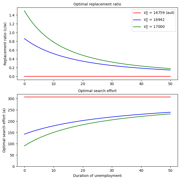
_images/d465929658695d7b57aca1ad1aeabff8c1004836bb2f2664f67c0721c4fd7cb6.png

For an initial promised value $V^{u} = V_{a u t}$ , the planner chooses the autarky level of $0$ for the replacement ratio and instructs the worker to search at the autarky search intensity, regardless of the duration of unemployment

But for $V^{u} > V_{a u t}$ , the planner makes the replacement ratio decline and search effort increase with the duration of unemployment.

40.4.2. Interpretations#

The downward slope of the replacement ratio when $V^{u} > V_{a u t}$ is a consequence of the planner’s limited information about the worker’s search effort.

By providing the worker with a duration-dependent schedule of replacement ratios, the planner induces the worker in effect to reveal his/her search effort to the planner.

We saw earlier that with full information, the planner would smooth consumption over an unemployment spell by keeping the replacement ratio constant.

With private information, the planner can’t observe the worker’s search effort and therefore makes the replacement ratio fall.

Evidently, search effort rise as the duration of unemployment increases, especially early in an unemployment spell.

There is a carrot-and-stick aspect to the replacement rate and search effort schedules:

the carrot occurs in the forms of high compensation and low search effort early in an unemployment spell.
the stick occurs in the low compensation and high effort later in the spell.

We shall encounter a related carrot-and-stick feature in our other lectures about dynamic programming squared.

The planner offers declining benefits and induces increased search effort as the duration of an unemployment spell rises in order to provide an unemployed worker with proper incentives, not to punish an unlucky worker who has been unemployed for a long time.

The planner believes that a worker who has been unemployed a long time is unlucky, not that he has done anything wrong (e.g.,that he has not lived up to the contract).

Indeed, the contract is designed to induce the unemployed workers to search in the way the planner expects.

The falling consumption and rising search effort of the unlucky ones with long unemployment spells are simply costs that have to be paid in order to provide proper incentives.